FLONGS
In this Flong one of the most famous dynamical systems will discussed, the logistic map. The logistic map is a one-dimensional discrete-time map that, despite its formal simplicity, exhibits an unexpected degree of complexity. Historically it has been one of the most important and paradigmatic systems during the early days of research on deterministic chaos.
The logistic map is defined by the following equation:
[ x_{n+1}=\lambda x_{n}(1-x_{n})\quad\text{with}\quad n=0,1,2,3… ]
Given a starting value $0\leq x_{0}\leq1$ and a positive parameter $0<\lambda<4$ the map produces a sequence of values
[ x_{0},x_{1},x_{2},… ]
that you get by iterating it, e.g.
[ x_{1} =\lambda x_{0}(1-x_{0}) ] [ x_{2} =\lambda x_{1}(1-x_{1}) ]
[ … ]
Panel 1: The sequence generated by the logistic map for a few values $x_n$. Change the initial value $x_0$ and the reproduction rate $\lambda$ with the sliders.
and so forth.
Before we discuss some fascinating properties of this map, its richness, and set of unexpected behaviors, let’s first motivate it and connect it to applications and natural systems.
Motivation
It turns out that the logistic map can be motivated using a biological/ecological context.
Let’s assume we have a population of a species in which individuals replicate. Let’s say, for simplicity that in every generation $n=0,1,2,…$ an individual has on average $\lambda$ offspring before it dies. This could be any positive number. It doesn’t have to be an integer because we think of this as an average or an expected number of offspring. So if say $\lambda=1.5$ then on average each individual has $1.5$ offspring in the lifetime of one time step, for instance if in 50% of cases an individual has one offspring and in 50% of the cases 2 children, we get $\lambda=1.5$.
We call the parameter $\lambda$ the reproduction rate.
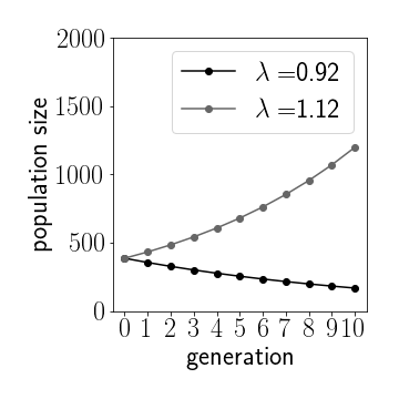
Figure 1: Depending on the growth rate we see exponential growth or decay. Initial population $U_0=400$
Now let’s say the population at time $n=0$ has $U_{n}$ individuals. A generation later the population size will be [ U_{n+1}=\lambda U_{n} ] Therefore, if we start with an initial population $U_{0}$ we get [ U_{n}=\lambda^{n}U_{0} ] which we can write as [ U_{n}=e^{\ln\lambda}U_{0} ] So, depending on the value of $\lambda$ we can have two different scenarios.
- If $0<\lambda<1$ then $\ln\lambda<\text{0}$ and thus $U_{n+1}<U_{n}$, the population dies out. This makes total sense if the typical number of offspring is less that one.
- If $\lambda>1$ on the other we have $\ln\lambda>0$ and thus $U_{n+1}>U_{n}$: the population grows indefinitely and exponentially.
So, if we only have replication and a reproduction rate $\lambda>1$ we expect exponential growth. Now, this can’t go on forever. Other factors will come into play if the population gets too big, e.g. limiting resources, competition, limited space, etc. One way to account for this is by saying that the reproduction rate $\lambda$ effectively depends in some way on the size of the population: [ \lambda=\lambda(U) ]
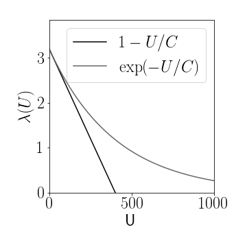
Figure 2: Two possible population size dependent reproduction rates $\lambda(U)$, linear and exponential decrease, respectively, for capacities of $C=400$ and basic reproduction rate $\lambda_0=3.2$.
We introduce a capacity $C$ which we think of as a large population size that, if reached, reduces reproduction to zero or a very small number. Plus we would like to keep reproduction at some maximum value $\lambda_{0}$ if $U\ll C$. What are the choices? Here’e one: [ \lambda=\lambda_{0}e^{-U/C} ] In this case [ \lambda\approx\lambda_{0}\quad\text{if}\quad U\ll C ] and [ \lambda\approx0\quad\text{if}\quad U\gg C ] An even simpler choice is a linear decrease [ \lambda=\lambda_{0}(1-U/C) ] which is very similar but potentially easier to handle mathematically.
With this choice we get [ U_{n+1}=\lambda_{0}(1-U_{n}/C)U_{n} ] which we can iterated for a chosen set of parameters $\lambda$ and $C$ and an initial population $U_{0}<C$.
Now we can simplify this a bit by expressing the population as a fraction of the capacity $C$: [ x_{n}=U_{n}/C. ] Using the new quantity we get [ x_{n+1}=\lambda_{0}(1-x_{n})x_{n}. ] We can just drop the subscript $0$ of $\lambda_{0}$ and arrive at the logistic map [ x_{n+1}=\lambda(1-x_{n})x_{n}. ]
Let’s play with this equation a bit. In Panel 2 you can observe the sequence $x_{n}$ for parameters $x_{n}$ and $\lambda$ of your choice. If $1<\lambda<3$ we get a sequence $x_{n}$ that quickly approaches a fixed value.
Panel 2: Time series of the logistic map. The sequence $x_n$ generated by the logistic map for a few values. Change the initial value $x_0$ and the reproduction rate $\lambda$ with the sliders. You can observe that for reproduction in the range $1<\lambda<3$ the solution approaches a stable fixed value. As you increase $\lambda$ a succession of period doubling events occurs.
If we increase the reproduction rate to $\lambda>3.0$ we observe a different behavior: The population doesn’t seem to equilibrate to a fixed value, but rather seems to oscillate in a period-2-cycle. Regardless of the initial condition $x_{0}$ the system always approaches this cycle.
Let’s go to even higher values. For $\lambda=3.8$ we see even for very long sequences no apparent regular or periodic pattern of values emerges. The sequence of values $x_{n}$ seems random and chaotic. More about this below.
One dimensional maps
In order to understand this behavior better, let’s back up a bit and think of a system like the logistic map in more general terms. The logistic map is an example of a one-dimensional discrete time map: [ x_{n+1}=f(x_{n}) ] where in our case [ f(x)=\lambda x(1-x). ] The question that arises typically is how the system behaves for long times so when $n\rightarrow\infty$.
Fixpoints
The first step we usually take is trying to identify special points, called fixed points or short fixpoints. These are values for $x$ that remain invariant if we plug them into the iterated map, so: [ x_{n+1}=x_{n} ] and [ x_{n}=f(x_{n}). ] Iterated maps can have none, one or many such points and sometimes it’s difficult to compute them. In our case we can compute the fixpoints: [ x=\lambda x(1-x) ] which has solutions [ x^{\star}=0 ] and [ x^{\star}=1-\frac{1}{\lambda}. ]
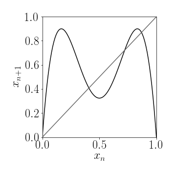
Figure 3a: Fixpoints of a 1-d iterated map $g(x)$ are the intersection of the function $g(x)$ with the diagonal. In this case the map $x_{n+1}=g(x_n)$ has 4 fixpoints.
We see that the first one always exists and the second one exists if $\lambda>1$. So if we start with $x_{0}=x^{\star}$ we will have [ x_{n+1}=x^{\star} ] for all times. But what happens if we don’t start with $x_{0}=x^{\star}$? Let’s try this with $\lambda=5/2$ and some $x_{0}$ we see that after a few iterations the values of $x_{n}$ are approaching the fixpoint [ x^{\star}=1-\frac{1}{\lambda}=3/5=0.6 ] This fixpoint seems to be attractive and we call it an attractor. Even if we start very close to the other fixpoint $x^{\star}=0$ say with $x_{0}=0.001$ we see that the values $x_{n}$ are repelled by it (we call that fixpoint a repeller) and attracted by the non-zero fixpoint.
Apart from doing the computations to determine the fixpoints we can find the fixpoints graphically. All we have to do is to draw the function $y_{1}=f(x)$ and the diagonal $y_{2}=x$. When these two curves intersect we have [ x=f(x). ] Therefore the intersections are the fixpoints, e.g. in Fig. 3a the map $x_{n+1}=g(x_n)$ has four different fixpoints.
For the logistic map we see that $f(x)$ is an inverse parabola that meets the $x$-axis at zero and one, and intersects with the diagonal $x$ only at $x=0$ if $\lambda<1$ and also at a non-trivial intermediate value if $\lambda>1$, consistent with the calculations we did, see. Fig. 3b.
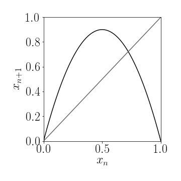
Figure 3b: Fixpoints of the logistic map are the two solutions to $x=f(x)$ which are the trivial fixpoint $x^\star=0$ and if $\lambda>1$ we also have $x^\star=1-1/\lambda$.
Stability
There’s a way to determine the stability of a fixpoint, to check whether a fixpoint is an attractor or a repeller. Let’s assume that we have a fixpoint $x^{\star}$. And we start off with an initial value that’s a little bit off so that [ x_{0}=x^{\star}+\delta x_{0}. ] Now we compute [ x_{1}=f(x_{0})=f(x^{\star}+\delta x_{0}). ] In the vicinity of the fixpoint, if $\delta x_{0}$ is very small we can expand the function $f$: [ f(x^{\star}+\delta x_{0})\approx f(x^{\star}) + f^{\prime}(x^{\star})\delta x_{0} ] so that [ x_{1} \approx x^{\star}+f^{\prime}(x^{\star})\delta x_{0} ] So, after one iteration, what is the distance to the fixpoint? [ \delta x_{1}\approx f^{\prime}(x^{\star})\delta x_{0}. ] So we see that if [ |f^{\prime}(x^{\star})|>1 ] this distance to the fixpoint becomes larger and larger whereas if [ |f^{\prime}(x^{\star})|<1 ] if becomes smaller and smaller. So it seems that this a condition for the stability of a fixpoint.
Let’s try to apply this to the logistic map. Here we have [ f(x)=\lambda x(1-x) ] which implies that [ f^{\prime}(x)=\lambda-2\lambda x ] so that at the fixpoint $x^{\star}=1-1/\lambda$ we get [ f^{\prime}(x^{\star}) =\lambda-2\left(\lambda-1\right) =2-\lambda ] Therefore, if $\lambda<3$ the fixpoint is stable because $|f^{\prime}(x^{\star})|<1$. But, if the reproduction rate increases beyond $3$ the fixpoint becomes unstable. The system no longer has a stable, attractive fixpoint.
Looking at the sequence $x_{n}$ say for $\lambda=3.3$ we see that the attractor is something else: a period-2-cycle of alternating values such that [ x_{n+2}=x_{n}=x_{A}^{\star} ] and [ x_{n+3}=x_{n+1}=x_{B}^{\star} ] We can think of both of these points that make that cycle as a fixpoint of a new map: [ g=f\circ f ] which in words means we apply the orginal map twice, or [ g(x) =f(f(x)) ] [ =\lambda f(x)(1-f(x)) ] [ =\lambda^{2}x(1-x)(1-\lambda x(1-x)) ] This function is a more convoluted polynomial. If we want to compute the fixed points of $g(x)$, we proceed the same way by solving [ x=\lambda^{2}x(1-x)(1-\lambda x(1-x)) ] for x.
Graphic Analysis - Cobwebbing
We can visualize a trajectory by starting on the $x$-axis at some point $x_{0}$ and drawing a vertical line to $f(x_{0})$. That point is also $x_{1}$ and finding it on the $x$ axis is equivalent to drawing a horizontal line towards the diagonal $x$. Now we can draw another vertical link to $f(x_{1})$ and keep repeating the process and eventually generate an entire trajectory this way. So, what we are doing is plotting the sequence [ (x_{0},0),(x_{0},x_{1}),(x_{1},x_{1}),(x_{1},x_{2})…. ] [ ….(x_{n},x_{n}),(x_{n},x_{n+1})…. ] You can try this cobwebbing for the logistic map in Panel 3.
Panel 3: Orbit reconstruction by cobwebbing. Two orbits are shown. You can vary the initial point $x_0$ for each orbit with the slider. An orbit has a transient period and an attractor. If you want to see the cascade of period doubling events, switch off the transient part of the orbit and increase the reproduction rate $\lambda$ slowly.
The road to chaos
So far we have observed that when $\lambda>1$ we have a single fixpoint at $x^{\star}=1-1/\lambda$ that loses stability at a critical value $\lambda_{2}=3$ when a stable period-2-cyle emerges. If we increase $\lambda$ beyond $\lambda_{3}=3.449…$ we will see that the period-2-cycle also loses stability. It is replaced by a new, stable and attractive period-4-cycle. The points that make up this cycle are stable fix-points of the quadruple map [ h=g\circ g=f\circ f\circ f\circ f. ] Now it turns out that this period-4-cycle doesn’t remain stable for long but at $\lambda_{4}=3.54409…$ is replaced by a stable period-8-cycle, and so forth.
What’s important to note is that the critical points at which these \textbf{period doubling events} occur, or rather there separation becomes smaller and smaller and eventually at [ \lambda_{\infty}=3.569946… ] we have a period of infinity. This means that although we have a ``cycle’' that is attractive, it’s period is infinite, so it never repeats, it is not longer really periodic. Rather is has become aperiodic and chaotic. This was very confusing to people that first looked at the simple logistic map. We can compute the ratio [ \delta=\lim_{k\rightarrow\infty}\frac{\lambda_{n}-\lambda_{n-1}}{\lambda_{n+1}-\lambda_{n}}=4.669 ] The limit is known as Feigenbaum’s constant. This is a universal constant that keeps reappearing in systems like the logistic map and is intimitaly connected to chaotic systems.
What’s even more puzzling is that the periodic solutions like the period-2-cycles, 4-cycles etc., although no longer stable in the chaotic regime, still exist as repellers. So for $\lambda>\lambda_{\infty}$ we have a very dense and infinite set of periodic orbits in the system all of which are unstable. In fact, they have to fit in the system somehow, so actually for every point $x$ we have an inifite set of periodic orbits arbitrarily close to it.
Bifurcation diagram
One way of illustrating the complexity of the situation is by what is known as a bifurcation diagram. Instead of making different cobwebbing plots for different choices of $\lambda$ and because we tend to be interested in the asymptotic behavior of the system we plot the attractors of the systems as a function of the parameter $\lambda$. A plot like this is known as a bifurcation diagram, a very important tool in the study of dynamical systems. This is how it works:
- first we fix $\lambda$ and choose an initial condition
- we then iterate the map, say 10000 times for the transient part of the dynamics
- then we iterating say 1000 more times and plot the array of values vs. $\lambda$
- we then increment $\lambda$ and repeat the process
we now plot the $x$-values that we computed that represent the attractor on the $y-$axis and the $\lambda-$value on the $x$-axis.
If for the chosen value of $\lambda$ we have say a period-8-cycle that is attractive, all the collected 1000 points will be one of the 8 points that make up the period-8-cycle. So we would get 8 dots in the plot. You can see what is happening in Panel 4.
Panel 4: The bifurcations in the logistic map. As we increase $\lambda$ a cascade of period doubling events leads to deterministic chaos. You can click on a region that interests you on the plot to zoom in around that region (After 6 zooming steps you will cycle back to the full display).
We clearly see the period doubling events as we increase $\lambda$. We also see that at some point all the points are spread across a wide range and form what looks like a continuun. Furthermore we see that there are weird self-similar structures in the bifurcation diagram and also regimes of periodic behavior within a see of chaos. You can investigate this by zooming by clicking on a region of interest.
Some properties of chaos
When the reproduction rate is larger than the critical parameter $\lambda_{\infty}$ and we have a regime where orbits are aperiodic, we have reached the regime of deterministic chaos. This means that even though the orbits are deterministic, they seem irregular and unpredictable.
We can also observe a sensitive dependence on initial conditions. Let’s say we start with an initial value $x_{0}$ and right next to it with an initial value $\tilde{x}_{0}=x_{0}+\varepsilon$ where $\varepsilon$ is tiny, say $10^{-6}$. In the chaotic regime after a few steps the sequences $x_{n}$ and $\tilde{x}_{n}$ will become very different, another hallmark of unpredictability. You can check this out in Panel 5.
Panel 5: Sensitive dependence on initial conditions. The figure depicts two orbits $x_n$ and $\tilde x_n$ differeing in their initial condition by a tiny bit $\varepsilon$. Increase the reproduction parameter $\lambda$ into the chaotic regime and you will see both trajectories diverge after a few iterations. Even if you then decrease $\varepsilon$ to a very small value, the number of steps for which both trajectories are similar doesn’t increase significantly.
Third, we see another generic feature of chaotic systems: self-similarity. This is particularly striking in the bifurcation diagram of Panel 4 where we see parts of the structure that resemble the whole structure only smaller. You can see this by zooming in (clicking on the region of interest).
Other systems
The logistic map with $f(x)=\lambda x (1-x)$ is the simplest conceivable system that encorporates reproduction and self-regulation of a population. Because it is so simple we can expect that models that are structurally similar but more realistic generate similar behavior and that the funky effects observed in the logistic map are universal.
Panel 6: Another bifurcation diagram. This one illustrates the bifurcations and period doubling of the map defined by $f(x)=\lambda x \exp (-x)$. Again click on a region of interest to zoom in.
Panel 6 illustrates the bifurcation diagram of the map
[ x_{n+1} = \lambda x_{n} \exp (-x_{n}) ]
which isn’t limited to a parameter range for the reproduction rate $\lambda<4$ but is plausible for any non-negative value. The bifurcation diagram looks qualitatively similar to the one depicted in Panel 4.
More material
A lot more can be said about the logistic map, one-dimensional non-linear maps in general, deterministic chaos and so forth. If you want to dive deeper into the material I suggest the following:
- The book on dynamical systems Nonlinear Dynamics and Chaos: With Applications to Physics, Biology, Chemistry, and Engineering by Steven Strogatz
- The seminal 1976 Nature paper Simple mathematical models with complicated dynamics by Bob May.